Hands-On Session: Math Camp Recap

Author

Rony Rodriguez-Ramirez

Published

04 September 2024

In this detailed hands-on session, we will walk through some fundamental data manipulation tasks in R using the starwars dataset from the dplyr package, covering essential functions for summarizing, filtering, arranging, and visualizing data. Throughout the session, we will practice different ways to compute summary statistics, filter data, and generate plots, focusing on applying both base R and tidyverse syntax. The goal is to consolidate what you learned during Math Camp while expanding on the key techniques for data analysis.

We start by loading the necessary libraries, specifically tidyverse, which offers a collection of R packages designed for data science. This package will allow us to manipulate and visualize data in a clear and concise manner.

library(tidyverse)

Next, Let’s calculate the total height of all characters in the dataset. We use the base R function sum to compute the sum of the height variable. This calculation includes the na.rm = TRUE argument to exclude missing values from the summation. Don’t worry thinking whether there is an intrinsic meaning or not to the output. We are doing this just for instructional purposes.

total_height <- sum(starwars$height, na.rm = TRUE)
total_height

[1] 14143

After obtaining the total height, we move to calculating the average height using the base R function mean. Again, the na.rm = TRUE argument ensures that missing values do not affect the calculation.

avg_height <- mean(starwars$height, na.rm = TRUE)
avg_height

[1] 174.6049

Now, we introduce the tidyverse syntax to achieve the same result, using the summarize function within a pipeline to calculate the average height. This approach is more readable and scalable for complex operations.

starwars |> 
  summarize(
    avg_height = mean(height, na.rm = TRUE)
  )

# A tibble: 1 × 1
  avg_height
       <dbl>
1       175.

Next, let’s compute the Body Mass Index (BMI) for each character by applying a transformation to the data. We use the mutate function to create a new variable, bmi, which is derived from the mass and height variables. Then, we select the characters’ names and their respective BMI values for display.

starwars <- starwars |> 
  mutate(bmi = mass / (height / 100)^2)

starwars |> 
  select(name, bmi)

# A tibble: 87 × 2
   name                 bmi
   <chr>              <dbl>
 1 Luke Skywalker      26.0
 2 C-3PO               26.9
 3 R2-D2               34.7
 4 Darth Vader         33.3
 5 Leia Organa         21.8
 6 Owen Lars           37.9
 7 Beru Whitesun Lars  27.5
 8 R5-D4               34.0
 9 Biggs Darklighter   25.1
10 Obi-Wan Kenobi      23.2
# ℹ 77 more rows

We can filter the dataset to identify tall characters whose height exceeds 200 cm. The filter function allows us to subset the data based on this condition.

tall_characters <- starwars |> 
  filter(height > 200)

tall_characters

# A tibble: 10 × 15
   name     height  mass hair_color skin_color eye_color birth_year sex   gender
   <chr>     <int> <dbl> <chr>      <chr>      <chr>          <dbl> <chr> <chr> 
 1 Darth V…    202   136 none       white      yellow          41.9 male  mascu…
 2 Chewbac…    228   112 brown      unknown    blue           200   male  mascu…
 3 Roos Ta…    224    82 none       grey       orange          NA   male  mascu…
 4 Rugor N…    206    NA none       green      orange          NA   male  mascu…
 5 Yarael …    264    NA none       white      yellow          NA   male  mascu…
 6 Lama Su     229    88 none       grey       black           NA   male  mascu…
 7 Taun We     213    NA none       grey       black           NA   fema… femin…
 8 Grievous    216   159 none       brown, wh… green, y…       NA   male  mascu…
 9 Tarfful     234   136 brown      brown      blue            NA   male  mascu…
10 Tion Me…    206    80 none       grey       black           NA   male  mascu…
# ℹ 6 more variables: homeworld <chr>, species <chr>, films <list>,
#   vehicles <list>, starships <list>, bmi <dbl>

Once we have the subset of tall characters, we sort them in descending order of height using the arrange function, and then display only their names and heights. The desc function ensures that the tallest characters appear at the top.

tall_characters |> 
  arrange(desc(height)) |> 
  select(name, height)

# A tibble: 10 × 2
   name         height
   <chr>         <int>
 1 Yarael Poof     264
 2 Tarfful         234
 3 Lama Su         229
 4 Chewbacca       228
 5 Roos Tarpals    224
 6 Grievous        216
 7 Taun We         213
 8 Rugor Nass      206
 9 Tion Medon      206
10 Darth Vader     202

We then perform grouping and summarizing to calculate the average height for each species in the dataset. The group_by function groups the data by species, and summarise computes the average height within each group.

avg_height <- starwars |> 
  group_by(species) |> 
  summarise(
    avg_height = mean(height, na.rm = TRUE)
  )

avg_height

# A tibble: 38 × 2
   species   avg_height
   <chr>          <dbl>
 1 Aleena           79 
 2 Besalisk        198 
 3 Cerean          198 
 4 Chagrian        196 
 5 Clawdite        168 
 6 Droid           131.
 7 Dug             112 
 8 Ewok             88 
 9 Geonosian       183 
10 Gungan          209.
# ℹ 28 more rows

In another example, we use group_by and mutate to create a new column mean_grouped, which stores the average height for each species directly within the dataset. This doesn’t modify the level of the dataset.

starwars |> 
  group_by(species) |> 
  mutate(
    mean_grouped = mean(height, na.rm = TRUE)
  )

# A tibble: 87 × 16
# Groups:   species [38]
   name     height  mass hair_color skin_color eye_color birth_year sex   gender
   <chr>     <int> <dbl> <chr>      <chr>      <chr>          <dbl> <chr> <chr> 
 1 Luke Sk…    172    77 blond      fair       blue            19   male  mascu…
 2 C-3PO       167    75 <NA>       gold       yellow         112   none  mascu…
 3 R2-D2        96    32 <NA>       white, bl… red             33   none  mascu…
 4 Darth V…    202   136 none       white      yellow          41.9 male  mascu…
 5 Leia Or…    150    49 brown      light      brown           19   fema… femin…
 6 Owen La…    178   120 brown, gr… light      blue            52   male  mascu…
 7 Beru Wh…    165    75 brown      light      blue            47   fema… femin…
 8 R5-D4        97    32 <NA>       white, red red             NA   none  mascu…
 9 Biggs D…    183    84 black      light      brown           24   male  mascu…
10 Obi-Wan…    182    77 auburn, w… fair       blue-gray       57   male  mascu…
# ℹ 77 more rows
# ℹ 7 more variables: homeworld <chr>, species <chr>, films <list>,
#   vehicles <list>, starships <list>, bmi <dbl>, mean_grouped <dbl>

To find the tallest species, we can arrange the summarized dataset by average height in descending order, extract the top entry, and use the pull function to display only the species name.

avg_height |> 
  arrange(desc(avg_height)) |> 
  head(1) |> 
  pull(species)

[1] "Quermian"

Finally, let’s use ggplot2 for visualization. First, we create a bar chart to display the tallest characters by height. The ggplot function initializes the plot, and geom_col adds the bars, with black borders and gray fill. We also use labs to label the axes and add a title to the plot, and theme_minimal to apply a clean, minimalistic theme.

tall_characters |> 
  ggplot(
    aes(
      x = height,
      y = name
    )
  ) + 
  geom_col(color = "black", fill = "grey") +
  labs(
    x = "Height",
    y = NULL, 
    title = "Tallest characters in Starwars"
  ) +
  theme_minimal()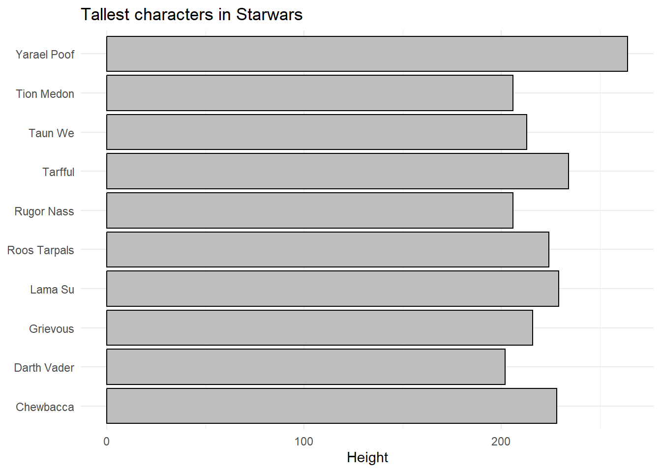

In another visualization, we reorder the character names by height using fct_reorder from the forcats package, ensuring that the tallest characters are displayed at the top of the plot. The structure is similar to the previous plot, but here we include reordering to enhance clarity.

tall_characters |> 
  mutate(name = fct_reorder(name, height)) |> 
  ggplot(
    aes(
      x = height,
      y = name
    )
  ) +
  geom_col(color = "black", fill = "grey") +
  labs(title = "Top 10 tallest characters in this dataset") +
  theme_minimal()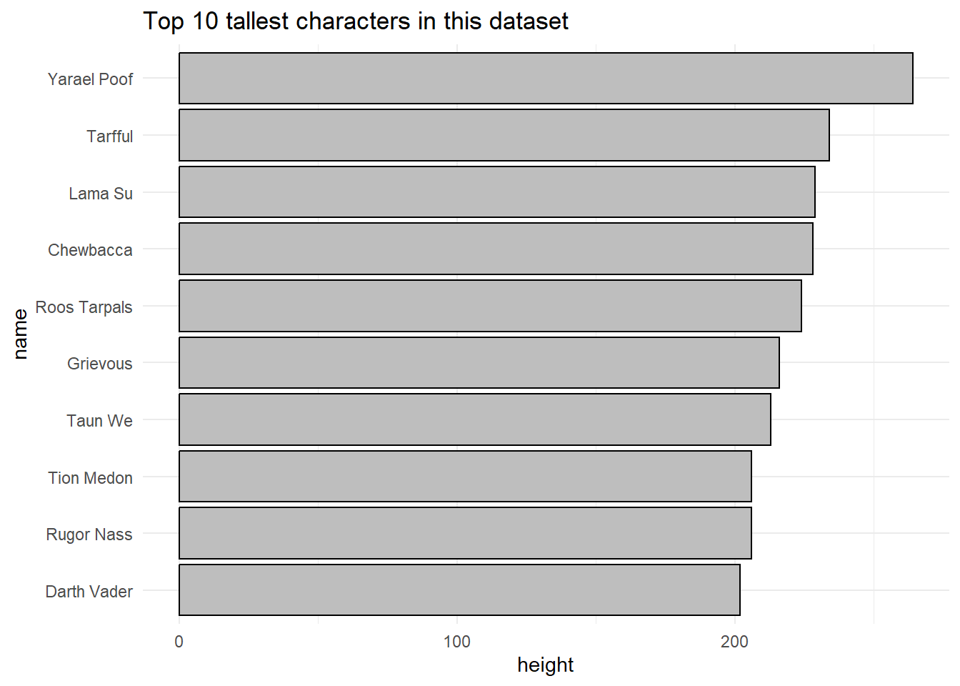

All the best with your first Problem Set!